Prodiams - Programmable Diagrams
The User Guide.
By Inspirel, rev. 1.1.
Contents
Prodiams were created out of frustration.
Prodiams are intended to allow engineers to work with diagrams and schematics following the same standards and processes that are already established in the world of software engineering:
Diagrams are specified by small and human-readable programs.
Those prorgams can be refactored and reused, archived in libraries and integrated with other useful code.
Diagrams are very easy to use in version-control and change-control systems, and they are diff- and patch-friendly. For the same reason, they are also easy to peer-review at the source level.
Prodiams were also intentionally made to be easy to generate or to act as sources for further processing, which makes them a versatile utility for model-based engineering and formal methods.
Prodiams is an open framework that can be extended with new layout rules and new shapes. For this reason, Prodiams is not supposed to be “complete” in any way - as such, it was meant to be in a state of continuous evolution.
System requirements
Prodiams is a framework created in the Wolfram programming language and is intended to be used in the Mathematica environment. The smallest known system that allows to work with Prodiams with reasonable level of comfort is Raspberry Pi.
“Hello World!”
This example is intentionally provided without any explanation:
Installation
As a software package, Prodiams is composed of (currently) three files:
Prodiams.wl - the base package defining most fundamental functionality, not tied to any particular engineering domain.
ProdiamsLogic.wl - extension of the base package with shapes for the most popular logic gates.
ProdiamsElectronics.wl - extension of the base package with shapes of several basic electronic components.
These files are expected to grow as new shapes and rules are added to them and new extensions packages are likely to be created to cover other engineering disciplines and notations.
For most comfortable use, all these files should be put in one of the directories defined by the $Path variable.
Loading the Prodiams packages
Prodiams packages are loaded as any other Mathematica package. Extension packages automatically pull the base package, so it is enough to load only the most specific package that is needed, for example:
![]()
or:
![]()
From now on, all Prodiams definitions (from base package and from extension packages) are available and the above commands will not be repeated any more.
Learning and getting help
This user guide itself is a Mathematica notebook and all examples in this guide are real - as such, they are immediately useful as a starting point for further modifications and learning by doing.
All Prodiams functions follow the standard Mathematica convention for documenting symbols and their descriptions can be retrieved in the usual way, for example:
![]()
![]()
Diagram’s anatomy
Every diagram is composed of shapes (like logic gates or electronics components, connecting lines, etc.), that are placed in the 2-dimensional coordinate system according to some set of layout constraints, which are hints regarding the placement of shapes.
These two ingredients are defined separately and can be even separately refactored and reused, but their interaction is what allows the final diagram to be created. In order to make it easier for the user to define diagrams, there are also some implicit rules that are always in action.
One of these implicit rules is that all shapes are drawn in the positive quarter of the coordinate system - that is, no shape is allowed to have negative coordinates, in both X and Y directions.
The other implicit rule is that there is a "gravity field" that attracts all shapes towards the origin of the coordinate system. This "gravity field" can be explained with the following plot:
The presence of this “gravity field”, with the implicit constraint that everything is kept on the positive side, means that if no rules are provided by the user, then all shapes will automatically fall to the bottom-left corner:
The “diagram” function is the main function creating diagrams and it accepts two arguments: the list of shapes to draw and the list of layout constraints to use. Above, the list of shapes contains two logic gates (“a” and “n”) and the list of layout constraints is empty, but thanks to the implicit rules described above, everything was attracted to the bottom-left corner.
The shapes are drawn in the order that they appear in the first list, which affects overlapping parts:
![]()
This can be a useful property in some types of diagrams.
In almost any realistic diagram, some layout constraints need to be added by the user to create meaningful visual structures:
![]()
Above, the “after” function is the layout directive that provides constraints for two shapes - the “n” shape is placed after (on the right of) the “a” shape. Still, since there are no rules acting in the vertical direction, everything falls to the bottom thanks to the ever-active “gravity field”.
It is easy to see that the NOT gate is somewhat lower than the AND gate, but this can be explained by the fact that for these shapes, the layout is computed for the connectors only - now it is clear that the lower input of the AND gate is at the same level as both input and output of the NOT gate; these are really Y=0 coordinate values. Similarly, both input connectors of the AND gate are at X=0.
There are layout directives operating in the vertical direction, too:
![]()
Of course, now both shapes are attracted to the left (all three input connectors are at X=0). If one shape needs to be placed both on the right and above another shape, then this expectation needs to be expressed with appropriate combination of layout constraints:
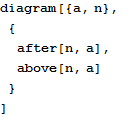
There are many more layout directives to help establish relative positions between shapes - “before”, “below”, “align”, “middle”, “center” and their variants working on whole lists. Some of them are used in later examples in this guide and all are listed in the Reference chapter.
Grid
In the diagrams above there was always a little bit of space left between shapes when “after” and “above” functions were used to establish their placement. This bit of space is not random and it is not fixed, either - but it is the first visible effect of another implicit constraint - that all coordinates are assigned natural values (no fractions).
This constraint can be visible here as well:
![]()
The “allAfter” directive is a shorthand for a series of “after” directives applied for each consecutive pair. All four dots were placed on consecutive available “nodes” in the imaginary grid of natural coordinate values - that is, “d4” was placed at X=0, “d3” at X=1, “d2” at X=2 and “d1” and X=3 - and for the lack of any vertical constraint, all four dots have Y=0 due to the presence of “gravity” that pulls everything towards the origin.
The space that is left between shapes can be controlled with the “offset” option that is 1 by default, but can have other (integer!) values as well:
The important property of the constraints managed with these functions is that the offset (default or explicit) has the meaning of “at least”, not “exactly”. This “soft” property allows multiple constraints to cooperate:
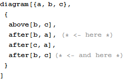
Above, directives marked by comments are not in conflict - “B” is after “A” at least 1 unit and it is also after “C” at least 1 unit. This cooperative property of layout directives allows easy modifications of the diagram when new shapes are inserted in between existing structures, which usually has only local impact and does not require the whole diagram to be redefined.
Point-like vs. composite shapes
Some shapes, like the dot from previous examples, have very simple structure and can be fully described by a single coordinate pair - these are point-like structures. Other shapes can have more complex nature and can have multiple coordinate pairs for their different components. The following example shows the difference:
Above, there are two shapes - one represents the “ground” symbol, which is very simple, and another for the transistor symbol with three connectors for base, collector and emitter. The presence of these connectors is what makes the transistor a composite shape, with multiple coordinate pairs. Logic gates from previous examples are composite, too.
The "connector" function allows to create a reference for a single point of the given composite shape - as such, this function itself returns some point-like structure (called “anchor”), which can be further used to create layout constraints. The simplest layout constraint is “pin”, which just forces two point-like structures to be at the same location - here the ground symbol is pinned to the transistor’s emitter connector.
Of course, the other transistor’s connectors have names “B” and “C” - and all three can be used in layout constraints:
Rigid vs. flexible shapes
Some composite shapes, like logic gates or transistors, have multiple points (connectors) with rigid structure between them. For example, the output connector of the logic NOT gate is always 8 grid units on the right of its input. These are rigid shapes as they define their own set of internal layout constraints.
There are other shapes, however, that are more flexible in nature and that allow the user to set up relations between their connectors. There are several two-connector electronics shapes that have this property:
Such shapes can be stretched and placed quite freely (with some reasonable limitations - only the connector lines are flexible, the core shapes themselves are not), but at the same time they require a bit more careful coding, because they cannot take care of themselves.
The above example also demonstrates that two-connector electronic shapes all have connectors named “A” and “B” and that if there is any notion of “direction” (voltage and current sources, diodes, polarized capacitors, etc.), it flows from “A” to “B”. Other shapes have connectors with more domain-specific names (like transistor’s “B”, “C” and “E”) or are completely user-defined (like with all logic shapes).
Labels
Most of the standard shapes support some form of labeling. For some of the shapes, like “inPort”, “outPort” and “block”, labels are essential and obligatory in the sense that they have to be provided as parameters when the shape is created:
![]()

Other shapes do not have any labels by default, but support them in a uniform way. For example, logic gates have inputs and outputs with user-provided names:
![]()
Above,”X” and “Y” are names that can be used to refer to input and output, respectively, for example in the “connector” function:
The connectors can have their own labels, though, and the easiest option is to automatically reuse connector names as labels:
![]()
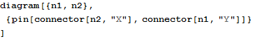
Connector labels do not have to be the same as their names:
![]()
The possibility to quickly label such shapes is especially convenient with shapes that have multiple inputs and outputs:
![]()
Shapes from the electronic family also support labels, but instead of labeling individual connectors (which usually have obvious meaning), there can be a single label per shape. The rules are similar as above:
Comments
Independently from labels, shapes can have comments that are displayed as tooltips when the mouse is hovered over them (obviously, this feature fully works only in the Mathematica notebooks, not in PDF, and HTML has only limited support for this feature):

Interestingly, comments are not limited to be text strings only - any Mathematica expression is fine, including plots and arbitrary images:
Styles
Prodiams have several ways to influence styling settings like line or fill colors.
There is a global association variable, named “defaultDiagramStyle”, that provides common settings for all diagrams:
![]()
| dotRadius→0.2 |
| roundingRadius→0.4 |
| labelFunction→Function[{t,point,align},{Black,Text[t,point,align]}] |
| gridSize→15 |
| diagramPadding→4 |
| printStats→False |
It is possible to change these values globally, which will affect all diagrams created from that point in time:
![]()
But for the sake of having stable foundations for the rest of this user guide, this setting will be reverted to its default value:
![]()
It is possible to override some (or all) of the settings with optional “style” setting in the diagram function and this affects only the given diagram:
![]()

It is also possible to provide such styling options when the shape is created - this way, the shape-specific settings will be used in all diagrams where that shape is used:
Above, "n2" has its own style, which is merged with default style settings whenever that shape is used. Such shape-specific styles have priority over diagram-specific styles (which themselves override default global styles).
As an ultimate way to override all other settings, the “styled” wrapper allows to define style options that override everything else. The following example demonstrates the complete hierarchy of style settings:
In the above example:
"n1" would have been "LightBlue" (due to default settings), but the diagram-level settings override it to "Red",
"n2" is “Green”, because it has its shape-specific style, which is more important than the diagram-level setting,
"n3" has the same specification as “n2”, but is “Blue” instead, because it was used within the “styled” wrapper that overrides all other settings.
Some of the style settings deserve additional explanation.
The "labelFunction” value in the style association denotes a function that can accept the same format of arguments as the standard Text function (the variant with offset arguments). In the simplest case it might be just set to Text, but there will be no control over font or its decoration. The anonymous function in the default setting shows a possible way to wrap the standard Text function with additional style directives. Of course, such function can be also defined separately, and - last but not least - actual mechanisms can be arbitrary and the provided function might do something else than just printing text.
The “gridSize” setting defines the size, in pixels in the final image, of the single grid unit. Changing this value has the effect of resizing all shapes:
![]()
The “diagramPadding” is an amount of white space, in grid units, that is artificially added around the whole diagram.
Finally, “printStats”, when set to True, allows to measure and print some performance statistics - this setting is useful only for debugging or for identifying performance optimization strategies with large diagrams.
Wrappers
Wrappers are functions that temporarily change some properties of their arguments - one such wrapper is the “styled” function from previous examples, that allows to locally override any style setting.
Another useful wrapper is the “hidden” function that suppresses the drawing of the given shape (or a list of shapes), while still using them for finding the layout solution - that is, the given shape still takes its space in the diagram, but is invisible, which allows to create several variants of the same diagram, showing different aspects of the same problem.
The following example can help demonstrate this concept:
![]()
![]()
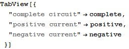
The “complete”, “positive” and “negative” are three diagrams that have exactly the same layout, but differ in the visibility of some of the shapes. Now it is easy to create a nice-looking viewer for all three variants:

The “styled” wrapper, explained above in the subsection devoted to style options, can also be used to achieve the effect of highlighting some aspects of the diagram like signal paths or important sub-modules.
Diagram refactoring
Some possibilities to refactor diagram definitions were already used above, where the longish sequence of layout constraints was assigned a separate name and that name was reused with three different diagrams - this definitely reduced the amount of code that would have to be written (or, worse, copy-pasted) otherwise. It would be also possible to refactor only some part of the sequence, or do similar simplifications in the list of shapes as well.
Such refactorings are very easy to do, but even more interesting effects can be achieved with parameterized functions.
The above diagram involves a common “impedance divider” pattern used in many different circuits and it makes sense to refactor this common pattern into a separate function:
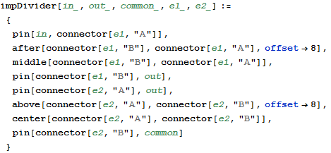
The “impDivider” function abstracts away the common design pattern and resolves to proper list of layout directives applied to shapes that are given as its parameters. Now the diagram definition can be much shorter:
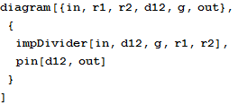

But a real benefit from this refactorization is that the same design pattern can be reused in other diagrams as well:
Or it can be even used multiple times within the same diagram:
Most importantly, such functions can be stored in a separate library or package and used as a common set of utilities - just as would be done in any reasonably managed project.
Semantics
The short version is: there is no semantics.
Prodiams allows to draw diagrams without any respect to whether they make sense or not. As such, it is just a drawing tool.
Interestingly, it is also possible to create diagrams that look reasonably well, but that do not convey the intended function:
Above, the two gates look like they are connected, but this is only a visual coincidence - the shapes are placed somewhere on the diagram and incidentally the connectors seem to be matched, but if that was the intention of the designer, it was not conveyed in the source code.
A much better way to express the design intent is to express it with “pin” directives:

This diagram looks the same as the previous one, but the sequence of layout directives contains information that can be extracted by otheer means and further processed or analyzed. In a bigger diagram, the set of “pin” instances can be sufficient to extract the complete connectivity map. It is recommended to follow this as a matter of good engineering practice.
Integration with Mathematica
Many of the examples in this guide already reached outside of the Prodiams package. Whether these are style settings referring to standard Mathematica color names or the possibility to create helper functions to refactor parts of the diagram - Prodiams work within the context of a much more versatile computing platform. Actually, considering the vast number of Mathematica functions, it would be difficult to name the limits of how much can be done.
The following example is definitely not meant to exhaust the subject, but hints at the possibility to write programs that generate diagrams:
The above diagram probably does not represent any reasonable system design, but is cool anyway and has high “management convincing potential”.
A more convincing example is included in the ProdiamsLogic package itself, in the form of the logicDiagram function that attempts to draw a reasonable diagram from the given logic expression:
![]()
Internally, the logicDiagram function decomposes the given expression and generates the list of shapes, together with appropriate layout constraints.
This chapter is intended for advanced users and explains the exact steps that are taken by the main engine in order to create the diagram. This description can be useful for those who would like to improve the framework or create new shapes.
The following, very simple diagram is dissected in this chapter:
As was already explained in earlier chapter, without user-provided layout constraint, everything would fall to the origin of the coordinate system due to the “gravity field” that is always active. In this context, user-provided constraints are additional equalities and inequalities that are added to the set of constraints and the solution is found for all involved coordinates.
The main engine learns about all involved coordinates by calling the “internalCoordinates” on all shapes:
![]()
![]()
The following shows the exact nature of what the “in” shape contributes:
![]()
{"in"["x"], "in"["y"]}
These are two expressions that are very readable for a human (even though this readability is not needed other than for debugging newly developed shapes), but from the Mathematica perspective they are not resolved and can be used as variable names. Intuitively, the “in” shape, being a point-like structure, contributes just two variables for its coordinates.
The output port “out” has similar set of coordinates, as it is also a point-like structure:
![]()
![]()
The resistor is a complex shape with two connectors and its set of coordinates reflects this:
![]()
![]()
Again, the “structure” of these expressions is irrelevant, although the “connector” function follows the same conventions:
![]()
![]()
![]()
![]()
The “connector” function creates an anchor object, which is an invisible point-like structure, referring to the same coordinates that the resistor reports on the list returned from “internalCoordinates”. It is therefore recommended to follow the same naming convention in newly developed shapes.
In any case, there are 8 variables involved in the whole diagram. Without any user-provided layout constraints, all these variables would be assigned 0 as a layout solution, which will be explained later on.
The layout constraints introduce relations between these variables. The “pin” directive is actually just a function that creates equalities for the coordinates of its arguments:
![]()
![]()
Similarly:
![]()
![]()
The “after” constraint is contributing some “stretch” to the whole structure:
![]()
![]()
These constraints express, in terms of coordinate variables, the relative positions of shapes, as intended in the use of the three directives - all layout directives just operate on coordinate variables, creating different equalities and inequalities.
What is important here is that layout constraints can be contributed not only by the user, but also by shapes themselves. Shapes communicate their own constraints by means of the “internalLayout” function - in this example, there are no such constraints:
![]()
![]()
The reason for this is that the shapes that are used in this diagram are either point-like structures (“in”, “out” - with just one coordinate pair there is no relation to contribute) or a flexible shape (resistor), which is set up by means of user-provided constraints. But there are also rigid shapes that have their own internal structure and can contribute their own constraints, for example:
![]()
![]()
![]()
![]()
Ultimately, it does not really matter where the constraints come from - both internal and user-provided constraints are merged together to create a single set of equalities and inequalities. This set is further extended by adding global constraints that keep everything in the positive quarter of the coordinate system:
![]()
![]()
![]()
![]()
This set of equalities and inequalities forms a solution space, where the minimum of the sum of all coordinates is found. The minimum of the sum of all coordinates is what creates the “gravity field” that pulls all variables towards the origin of the coordinate system:
![]()
![]()
It should be now obvious why, without any user-provided constraints, all shapes would fall to the origin of the coordinate system - this is where the above function has its minimum. But user-provided constraints, which usually affect relative placement of shapes, expand the solution further apart.
The actual workhorse of the Prodiams package, and the central point of the “diagram” function, is the Minimize function, which is called like this (taking into account above expressions):
![]()
The first value above is the value of the goal function, which is discarded (who cares what is the sum of coordinates?) and the second part is the actual solution. This solution is then fed to the “draw” function that is called for each shape, which also accepts the hierarchically merged style settings. As a funny example, the following is the list of graphics primitives that “draw” returns for the resistor in this diagram:
![]()
![]()
As can be seen from the last elements in this list, the resistor shape in this diagram extends from {0,0} to {8,0}, which corresponds to the solution for its coordinate variables.
All such contributions, from all involved shapes, are combined and the final graphics is created:
![]()
As a final touch, the main engine checks the “boundingBox” of all involved shapes, which allows to determine the extent of the whole diagram, so that proper padding and plot range can be selected. Image size is determined from “gridSize” style setting and the extent of the complete diagram.
That’s it!
The above explanation can be helpful for those who would like to extend the framework or develop new shapes - in which case the important take-away from the above is that each new shape needs to implement the following functions:
“internalCoordinates” - returns the list of coordinate variables for the given shape; the existing naming convention should be preserved to benefit from some of the existing helper functions,
“internalLayout” - returns the shape’s contribution to the list of coordinate constraints; this list can be empty for point-like structures and flexible shapes that rely on user-provided constraints for their layout,
“specificStyle” (not used above) - returns the set of shape-specific style options; these values are merged with default and diagram-specific settings,
“boundingBox” - returns the Rectangle-like coordinates (bottom-left - top-right) of the shape’s extent,
“draw” - returns the list of graphics directives and primitives for the given shape, layout solution, and style settings.
Of course, the existing shapes can be used as a reference and a source of code patterns to reuse.
List of layout directives
All layout directives are defined in the base Prodiams package.
List of wrappers
All wrappers are defined in the base Prodiams package.
List of shapes
Prodiams (base package)
ProdiamsElectronics (extension package)
ProdiamsLogic (extension package)
Shape API
Shape API is a set of functions that allow interactions between main diagrams engine and (newly developed) shapes.
Note: all these functions are first used in the base Prodiams package and their implementations for new shapes need to be kept in the base context, even if shapes themselves are implemented in other (extension) packages.
Optionally, for composite shapes that have the notion of connection points: