


|
|
||
|
Automatic proofs of statements derived and describing some chosen program properties are probably the most effective (like in “spectacular”) tool in the formal methods family. Many such statements are automatically generated based on existing model definitions - for example, checks that computed values fit their intended target type - others, like pre- and post-conditions or in-code assertions can be explicitly added by the engineer to mark his design intents.
Some introduction to the terminology used in FMT is in order, before explaining proof check features in detail.
Engineers working with imperative programming languages are used to the concept of sequential execution flow and the fact that program effects like modification of object values happens one after another on the program execution path. For example, in the following snippet:

there is no confusion with regard to the value that x and y have at the end - the initial conditions are straightforward and following the consecutive changes is relatively easy.
Things become more complex when it is necessary to backtrack such modifications in order to find answers to questions like "can a given state be reached"? This example demonstrates the problem:
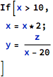
In the code above it might not be possible to find the exact values that x and y have at the end, but it might be still necessary to find out whether the code has a division by 0 error. This can be checked by solving a simple set of equations or inequalities, with a bit of preparation work. Namely, since the value of x is modified in the middle of the calculation, there is a need to represent it differently for each state it has during the whole sequence of statements. The example set of inequalities here can be:

Since it is necessary to refer to variable x twice to represent its two different states, effectively the whole calculation is turned into a two-variable problem. This problem has no solution, so it can be concluded that it is not possible to divide by 0 and therefore this particular code fragment is safe.
Creating new variables to represent different versions of objects that have their values updated by consecutive statements is called “freezing”. Consecutive freezes create new variables that have their original name retained with subscripts representing the “version number”. Longer sequences of assignments and updates create more frozen versions, for example the following sequence of assignments:

leads to this set of equalities:

Such a set retains all intermediate values, which can also make it easier to follow the individual calculation steps.
The example snippet above already indicated that there exists a process of cumulation of statements for use in creating more complete problems. Indeed, statements are accumulated from the very beginning of the operation, for each possible control path separately. It is also assumed that previous problems have been already solved, so that further ones can rely on checks that were already done. Those statements that were accumulated so far (at any given point in the execution path) are “knowns” and those that are yet to be checked are considered “expectations”. Expectations join the set of knowns for problems encountered further down the execution path. Thus, in the earlier snippet, when the division by 0 problem is solved, the following are “knowns”:

and the following is to be checked:

This distinction is not relevant from the point of view of the given set of equalities and inequalities, as all statements are taken together anyway, but is useful for readability when statements are listed for inspection and diagnostics.
Some statements become “knowns” by their very nature - operation pre-conditions, type invariants for package-level data objects or operation input parameters and branch conditions in conditional statements (like in the If statement above) are taken as “knowns” immediately as they are encountered. On the other hand, correctness conditions like denominator not being zero, type invariants for newly computed values and operation post-conditions are “expectations”, which are checked by means of solving appropriate problem sets, like in the example above.
A dedicated reference chapter lists all knowns and expectations that are generated by FMT.
Initialization of local variables as well as updates of inOut and out parameters is the aspect of data flow analysis that is covered by proof checks. In order to enable this, additional variables are automatically introduced to track the initialization state of such objects, including their frozen versions. For example, for a variable x its initialization flag has the following name:

Such variables are added to the set of “knowns”. Initialization flags are Boolean variables that are True or False depending on whether their respective variable was initialized or not. For the freshly created local variable x, its initialization state is expressed as:

which can be read as: “variable x was not initialized”.
However, after the variable is assigned to and its new frozen version is created, the initialization state is also versioned and added to the set of “knowns” as:

which can be read as: “first update of x was initialized”.
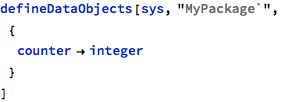
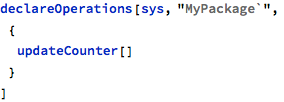
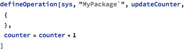
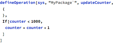
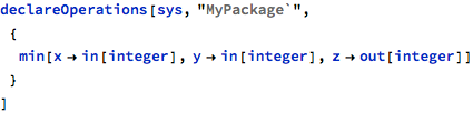
The following example demonstrates a simple operation that is supposed to count its invocations using a package-level counter object to keep state across calls:
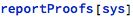
The updateCounter operation (in fact, the whole model) can be verified by means of proof checks with the following command:

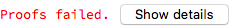
The checks, which were invoked for the whole model, failed - this means that some of the operations within the model were found to be incorrect. The “Show details” button allows to display them:
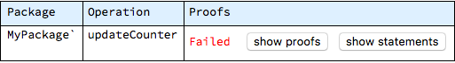
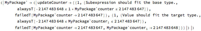
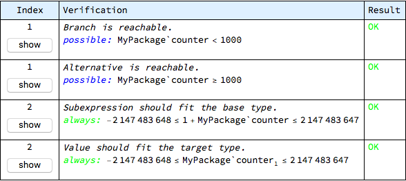
The information that is gathered during proof checks is conveniently divided into two groups, which can be separately inspected with the help of buttons displayed for problematic operations. The “show proofs” button can be used to focus on verification results only, while keeping the detailed context of each check aside. In the case of updateCounter operation, two checks are generated and both of them fail:
The same table can be displayed directly with:

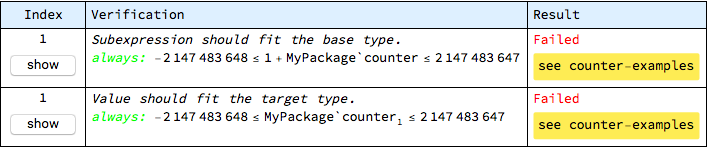
There is a seeming duplication in this report, which results from the fact that subexpressions and assignments are checked separately. In this case the first item on the list is the only one that needs to be addressed and its complete breakdown is as follows:
The problem was found in the first statement of the updateCounter operation. The “show” button in first column of the table allows to display the control flow diagram with highlighted location of the problem:
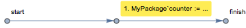
It is clear that the offending operation is the assignment to the package-level counter object.
A human-readable description of the verification check, in the second column, is:

Each condition that is automatically generated has an associated description - in this case the expectation is that calculations performed in individual subexpressions should produce results that stay within the range of the base type, which is integer here. The subexpression in question is:

This calculation should stay within the range of the base integer type.
The green “always” word below the description indicates the kind of verification check - its meaning here is that the given condition needs to be true for all possible runs of the operation. Other kinds of verification checks are “never” (printed in red, for example denominator must never be zero) and “possible” (printed in blue, for example it should be possible, but not necessary, for the conditional branch to be entered).
The last piece displayed in the second column of the table is the actual statement that becomes part of the solved set. Here the statement is:

This statement is derived from the default (and configurable) range of the integer type, which is supposed to be 32-bit, signed.
In summary: adding 1 to the current value of counter should not overflow the integer type.
This verification goal has failed, which is reported in the third column of the table. The highlighted link named “see counter-examples” displays, in the form of a tooltip, the possible combination of variable values that makes the verification goal failing - here the counter-examples are:

The meaning of this is that if the counter object has this value at the beginning of the operation, then the expression will overflow - indeed, the numeric value shown is the default upper limit for the integer type, so it is not possible to increment it and since there is nothing in this particular operation that would prevent such initial state when the operation is invoked, the possibility is considered real.
The second row of the table refers to the assignment operation itself, which involves the whole calculation. The seeming duplication is related to the fact that the calculation involves exactly one subexpression, which is already dealt with in the first row of the table.
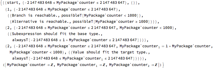
As with all other FMT functions, the same report exists also in the raw format, as a nested Association object:
The part that requires explanation here is the failedT tag, which wraps all counter-examples - it would be provenT[] in case of successful check. The tag alwaysT, or its siblings neverT and possibleT, are used to describe the kind of respective verification statement.
Similarly to other functions that perform checks for multiple operations, both showProofChecks and reportProofs functions accept options for selective choice of analyzed operations, for example:

By default the whole model is analyzed.
The updateCounter operation can be fixed by implementing a simple saturation scheme, where the value is no longer incremented after reaching some arbitrary limit:
After this correction the proof check results are now correct:

The detailed results can be still displayed with the showProofResults function, but this time, due to the fact that the operation body is more complex, more checks are generated:

The interpretation of this report should follow the same scheme as before. Those entries that are new with regard to the previous report are related to the conditional If statement, which is now statement number 1. For each conditional expression the condition itself is checked for whether it is effective at all - the condition is considered useful if it is possible for that condition to be True in some program runs and False in others. For If statements that have both “then” and “else” branches the meaning of this check is intuitive, as it verifies whether both branches are reachable, otherwise they would be just dead code. In this program, however, the If statement has no “else” branch - yet, the check for alternative branch (that is, for the condition to be False) is still useful, because it ensures that the conditional statement is not redundant and it does indeed introduce alternative execution paths. Similar checks are generated for other conditional constructs as well.
In this corrected program version all checks are successful. This verifies that there are no computation overflows, for every imaginable program run.
The analysis of such cases can be easier when the verification checks are shown together with all “knowns” that provide the context for checks. Such bigger context allows to better understand how the given proof problem is constructed and, perhaps, to find out that it is not sufficient for automated proof - in other words, that it is underspecified, even though the engineer might have additional knowledge that allows him to positively review the given code. Such underspecified context can be enriched with more explicit definitions - in terms of type invariants, pre-conditions or assumptions.
The whole proof context for all execution steps in any given operation can be displayed with the "show statements" button, which was displayed at the beginning of this example (when there still were errors) or explicitly with the following command:

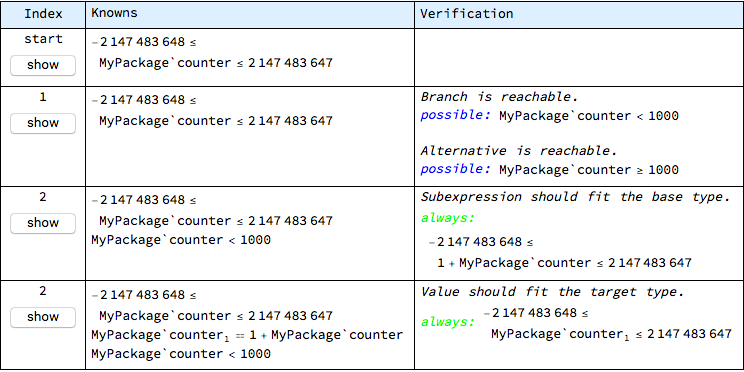
This table is different from the previous one in that there are no check results. In fact, this table is not concerned with whether the checks pass or fail.
What this table reveals is, aside each check, the “history” of context accumulation on every execution path. This history can be inspected and validated by a human reviewer as a confidence check for the soundness of the whole proof process. If some important information is missing from this table, the model might require more details in its specification.
An interesting additional row in this table describes the “knowns” at the very beginning of the operation body, before any statement is reached - this is at the virtual “start” index, where the only things that are known are operation pre-conditions and type invariants of involved objects. In this case, the object counter, which is a package-level object, is considered to be already initialized and so it is known that its value fits in the range of its type.
The same report is available in the raw format, for algorithmic processing:

The data structure reported this way is a pair, which first element is a list of reports (triples) corresponding to rows in the table above and the last element is an association object defining domains for all involved variables. In this example all variables are consecutive versions of the counter value and their domain is Integers.
As the execution path progresses through the operation body (including branches, if there are any), the list of “knowns” becomes longer. Such a breakdown makes it relatively easy to diagnose errors reported in the other table.
Another simple example presents how the versioning interacts with initialization tracking and how the model can be enriched to add missing design knowledge. In this example, the min operation returns, by means of its out parameter, the minimum of the first two parameters:
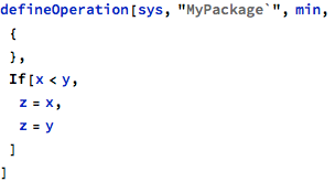
The whole proof context for consecutive steps of this operation can be displayed with:

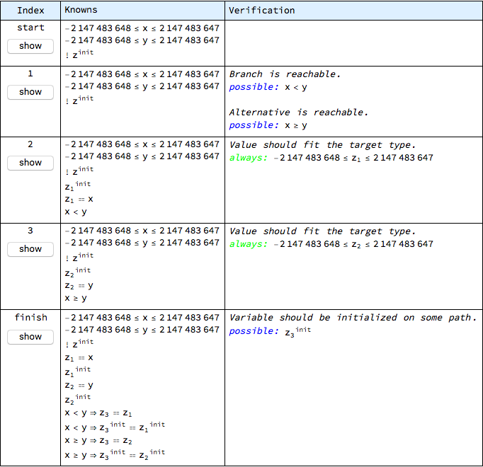
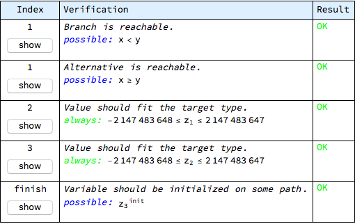
All checks prove correct in this operation:

In particular, z is proven to be initialized by checking that it is possible for the following to be True:

The context displayed in the previous table allows to perform a hand-verification of this conclusion, but at the same time it can be noticed that the initialization of z is not obligatory - it has the “possible” category, instead of “always”. This is the default meaning of out parameters, which can be justified by operations like search or lookup, where the searched for element might or might not be found. This default meaning might not correspond to the design intent of the min operation, where it is too weak.
The promise that z is always updated can be expressed explicitly in the operation post-condition:
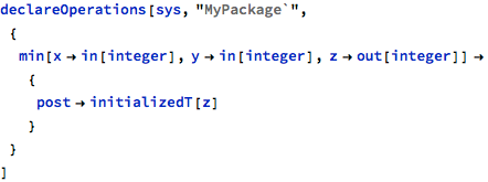
The initializedT wrapper is an internal representation of the initialization flag. Such a post-condition is added to the list of checks, with appropriate (the last available) version chosen for z:

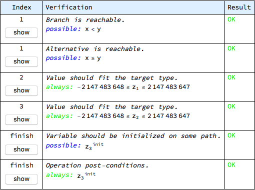
The lats check in this table comes from the explicit post-condition. It is also proven correct, which makes sure that the min operation always updates its output parameter.
The above example is a bit artificial in that a more complete post-condition that describes the expected value of the z parameter would also automatically ensure that it is properly assigned to and then referring to the initialization state of that parameter would not be necessary. Still, the possibility to control the “promise to update” property can be useful.
Previous: Data aliasing checks, next: All checks
See also Table of Contents.